CS4215 Project Report

Title: Explicit-control evaluator (ECE) for Go

Team Members: Rama Aryasuta Pangestu (A0236444E), Yeung Man Tsung (A0255829N)

Repository URL: https://github.com/benson1029/go-slang

Live Demo: https://benson1029.github.io/go-slang/

Presentation Slides: CS4215_Presentation_Slides.pdf

This report can be viewed online on https://benson1029.github.io/go-slang/docs/project-report/report.

Table of Contents

• CS4215 Project Report
  • Table of Contents
  • Project Objectives
  • Language Processing Steps
  • ECE Specification
    • Instruction Set
      • Helper Instructions
      • Expressions
      • Variables
      • Control Flow
      • Functions
      • Constructors
      • Arrays
      • Structs
      • Slices
      • Goroutines and Channels
    • State Representation
    • Inference Rules for Selected Parts
      • Helper Instructions
      • Expressions
      • Variables
      • Sequence and Block
      • For Loop
      • Go Function Call
      • Mutex Lock and Unlock
      • Channel Send and Receive
      • Select Statement
  • Project Source
  • Test Cases

Project Objectives

We implement an explicit-control evaluator (ECE) for the following subset of the Go programming language:

• Sequential constructs: Variable declarations and assignments, expressions, control flow (if, for), functions, and complex types (strings, structs, arrays, slices).
• Concurrent constructs: Goroutines, mutex, wait groups, channels, and select statements.

Additionally, we implement a low-level memory management system with both reference counting and mark-and-sweep garbage collection. All data structures, including control stack, heap, and environments, are stored in a single array buffer. We also implement a visualizer for the ECE machine.

All objectives are met in the final implementation. However, the following language features are not in scope:

• Sequential constructs: switch statements, defer statements, and panic and recover functions. Anonymous structs, indexing and slicing of strings, pointers, maps and tuples are also not implemented.
• Concurrent constructs: Closing of channels is not implemented.

The exact subset of the Go programming language that we support, along with some examples, can be found in the language specification page.

Language Processing Steps

Externally, this ECE machine is an interpreter for Go written in JavaScript, which is then run in a JavaScript interpreter (the browser). This is shown using the following T-diagram:

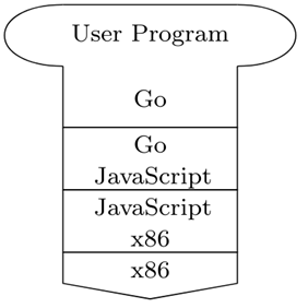
Internally, the Go program is first parsed into an abstract syntax tree (AST) using a parser, generated with peg.js using our own syntax definition. The AST is then preprocessed by a preprocessor, which annotates the global scope declarations with their necessary captures and then sorts the global scope declarations such that their dependencies are satisified. The preprocessed AST is then passed to a loader, which loads the entire program into the heap and initializing the Control stack in the ECE machine. The ECE machine then executes the instructions in the Control stack.

ECE Specification

Instruction Set

The following tables show the instruction set of the ECE machine.

Helper Instructions

Instruction	Description	Parameters	Stash
PUSH_I	Pushes a value into the stash	value (value)	None
POP_I	Pops a value from the stash	None	value (value)

Expressions

Instruction	Description	Parameters	Stash
BINARY	Performs a binary operation (includes logical operations)	operator (string), left_operand (rvalue expression), right_operand (rvalue expression)	None
BINARY_I	Performs a binary operation	operator (string)	None
LOGICAL_IMM_I	Performs a logical operation with only the left operand in the stash	operator (string), right_operand (rvalue expression)	left_operand (value)
LOGICAL_I	Performs a logical operation with only the right operand in the stash	operator (string)	right_operand (value)
UNARY	Performs a unary operation	operator (string), operand (rvalue expression)	None
UNARY_I	Performs a unary operation	operator (string)	None
LITERAL	Pushes a literal value into the stash	type (string), value (value)	None

Variables

Instruction	Description	Parameters	Stash
ASSIGN	Assigns a value to a variable	name (lvalue expression), value (rvalue expression)	None
ASSIGN_I	Assigns a value to a variable	None	name (address), value (value)
VAR	Declares a variable with an initial value	name (string), value (rvalue expression)	None
VAR_I	Declares a variable with an initial value	name (string)	value (value)
NAME	Accesses the value of a variable	name (string)	None
NAME_ADDRESS	Accesses the address of a variable	name (string)	None

Control Flow

Instruction	Description	Parameters	Stash
SEQUENCE	Executes a sequence of instructions	body (linked list of instructions)	None
BLOCK	Starts a scope, i.e. pushes a new environment frame	body (sequence)	None
EXIT_SCOPE_I	Exits the current scope, i.e. pops the environment frame	None	None
IF	Conditional statement	condition (rvalue expression), then_body (block), else_body (block)	None
IF_I	Conditional statement	then_body (block), else_body (block)	condition (boolean)
FOR	Iterative statement	init (statement), condition (rvalue expression), update (statement), body (block)	None
FOR_I	Iterative statement	condition (rvalue expression), update (statement), body (block), loopVar (name or null)	condition (boolean)
MARKER_I	Marker to signify the end of the loop body	None	None
BREAK	Breaks out of the loop	None	None
CONTINUE	Continues to the next iteration of the loop	None	None

Functions

Instruction	Description	Parameters	Stash
FUNCTION	Declares a function	name (string), param_names (array of strings), capture_names (array of strings), body (block)	None
CALL	Calls a function	function (rvalue expression), args (array of rvalue expressions)	None
CALL_I	Calls a function	num_args (int)	function (value), args (array of values)
CALL_STMT	Calls a function and discards the return value	body (a CALL instruction)	None
RETURN	Returns a value from a function	value (rvalue expression)	None
RETURN_I	Returns a value from a function	None	value (value)
RESTORE_ENV_I	Restores the environment frame before the function call	frame (environment frame)	None

Constructors

Instruction	Description	Parameters	Stash
DEFAULT_MAKE	Pushes the default value of a type into the stash	type (string), args (array of any)	None
MAKE	Constructs a value of a type according to the make function call	type (string), args (array of rvalue expressions)	None
MAKE_I	Constructs a value of a type according to the make function call	type (string), num_args (int)	args (array of values)
CONSTRUCTOR	Constructs a value of a type according to the initializer list {...}	type (string), args (array of rvalue expressions)	None
CONSTRUCTOR_I	Constructs a value of a type according to the initializer list {...}	type (string), num_args (int)	args (array of values)

Arrays

Instruction	Description	Parameters	Stash
INDEX	Accesses the value of an array element	array (rvalue expression), index (rvalue expression)	None
INDEX_I	Accesses the value of an array element	None	array (value), index (value)
INDEX_ADDRESS	Accesses the address of an array element	array (rvalue expression), index (rvalue expression)	None
INDEX_ADDRESS_I	Accesses the address of an array element	None	array (address), index (value)

Structs

Instruction	Description	Parameters	Stash
STRUCT	Declares a struct	name (string), fields (array of names and types)	None
METHOD	Declares a method for a struct	struct_name (string, name of the struct), name (string), self_name (string), param_names (array of strings), capture_names (array of strings), body (block)	None
MEMBER	Accesses the value of a struct member	object (rvalue expression), member (string)	None
MEMBER_I	Accesses the value of a struct member	None	object (value), member (string)
MEMBER_ADDRESS	Accesses the address of a struct member	object (rvalue expression), member (string)	None
MEMBER_ADDRESS_I	Accesses the address of a struct member	None	object (address), member (string)
METHOD_MEMBER	Accesses the value of a method member, and pushes the current object into the stash (for the method call to use)	object (rvalue expression), member (string) , struct (string, name of the struct, annotated during type checking)	None

Slices

Instruction	Description	Parameters	Stash
SLICE	Slices an array	array (rvalue expression), start (rvalue expression), end (rvalue expression)	None
SLICE_I	Slices an array	None	array (value), start (value), end (value)
SLICE_ADDRESS	Slices an array	array (rvalue expression), start (rvalue expression), end (rvalue expression)	None
SLICE_ADDRESS_I	Slices an array	None	array (address), start (value), end (value)

Goroutines and Channels

Instruction	Description	Parameters	Stash
GO_CALL_STMT	Calls a function in a new goroutine	body (a CALL instruction)	None
GO_CALL_I	Calls a function in a new goroutine	num_args (int)	function (value), args (array of values)
CHAN_RECEIVE	Receives a value from a channel	channel (rvalue expression)	None
CHAN_RECEIVE_I	Receives a value from a channel	None	channel (address)
CHAN_RECEIVE_STMT	Receives a value from a channel and discards it	body (a CHAN_RECEIVE instruction)	None
CHAN_SEND	Sends a value to a channel	channel (rvalue expression), value (rvalue expression)	None
CHAN_SEND_I	Sends a value to a channel	None	channel (address), value (value)
SELECT	Selects a case from a list of cases	cases (array of cases)	None
SELECT_I	Selects a case from a list of cases, with the expressions already evaluated	select (a SELECT instruction)	The evaluated expressions for all cases
CASE_SEND	A case for sending to a channel	channel (rvalue expression), value (rvalue expression), body (sequence)	None
CASE_RECEIVE	A case for receiving from a channel	channel (rvalue expression), assign (null or lvalue expression), body (sequence)	None
CASE_DEFAULT	A default case	body (sequence)	None

State Representation

info

$\cdot \mathbin\Vert \cdot$ denotes the concatenation of two elements. For example, $x \mathbin\Vert y$ is the concatenation of $x$ and $y$. In particular, $x \mathbin\Vert \varnothing = x$, $\varnothing \mathbin\Vert y = y$, and $\varnothing \mathbin\Vert \varnothing = \varnothing$.

The ECE machine has the scheduler $\mathcal{T} = T_{i_1} \mathbin\Vert T_{i_2} \mathbin\Vert \ldots$, where $T_{i_1}, T_{i_2}, \ldots$ are the (unblocked) threads in the scheduler. Each thread $T_i$ is a tuple $(C, S, E)$, where $C$ is the control stack (containing instructions), $S$ is the stash (containing runtime values for instructions), and $E$ is the environment.

The control stack and the stash are represented as the concatenation of its elements $x_1 \mathbin\Vert x_2 \mathbin\Vert x_3 \mathbin\Vert \ldots \mathbin\Vert x_k$. The environment is a tuple $E = (\Delta_N, \Delta_S)$, where $\Delta_N$ and $\Delta_S$ are the name and struct frames, respectively.

• $\Delta_N$ is a concatenation of environment frames $\Delta_1 \mathbin\Vert \Delta_2 \mathbin\Vert \ldots \mathbin\Vert \Delta_n$, where each environment frame $\Delta_i$ is a hash table that maps variable names to its address in the heap.
• $\Delta_S$ is a hash table that maps struct names and methods to their addresses in the heap. Currently, we only support struct declarations on the global scope, so there is a single struct frame $\Delta_S$ for the entire program.

A variable $x$ is a pointer to a value $v$ in the heap (the value for the variable). Therefore, a variable will have a fixed address $a$ in the heap. When a variable is inserted into an environment frame, the environment frame hash table keeps a mapping from the variable name (represented by a string object in the heap) to its fixed address $a$ in the heap.

We define the following operations on the environment:

• $\varnothing \mathbin\Vert \Delta$ is the environment frame $\Delta$ with a new empty child frame.
• $\Delta[x \gets v]$ is the environment frame $\Delta$ with the variable $x$ bound to the value $v$.
• $\Delta(x)$ is the value bound to the variable $x$ in the environment frame $\Delta$.
• $\Delta(x)_a$ is the address of the variable $x$ in the environment frame $\Delta$.

If we update the value of an object in address $a$ to a new value $v$, this change is reflected in all threads that have a reference to the address $a$. As this is a global change, we denote this operation as $\mathcal{H}[a \gets v]$, where $\mathcal{H}$ is the heap. Similarly, we can denote $\mathcal{H}(a)$ as the value at address $a$ in the heap.

However, it's not just the values of environment variables which are stored in the heap. The scheduler $\mathcal{T}$, each of its threads $T_i = (C_i, S_i, E_i)$, the control stack $C_i$, the stash $S_i$, and the environment $E_i = (\Delta_{N_i}, \Delta_{S_i})$ are all stored in the heap. We denote the address $\mathcal{T}_a$ of the scheduler in the heap such that $\mathcal{H}(\mathcal{T}_a) = \mathcal{T}$.

Therefore, since all objects determining the state of the ECE machine are stored in the heap, we have the following state representation:

info

The state of the ECE machine is the heap $\mathcal{H}$.

For clarity, however, we will slightly abuse notation and denote the state of the ECE machine as $(\mathcal{T}, \mathcal{H})$, where $\mathcal{T} = \mathcal{H}(\mathcal{T}_a)$. It is important to remember that this is a shorthand notation to easily refer to the scheduler $\mathcal{T}$, and the actual state of the ECE machine only depends on the heap $\mathcal{H}$.

This shorthand notation allows us to treat $\mathcal{T}$ as if it's a separate entity from the heap $\mathcal{H}$, but note that any changes to $\mathcal{T}$ are also reflected in $\mathcal{H}$. In other words, we can view $\mathcal{T}$ in $(\mathcal{T}, \mathcal{H})$ as a (mutable) reference to the scheduler object $\mathcal{H}(\mathcal{T}_a)$ in the heap $\mathcal{H}$. Implicitly, we treat the children of the scheduler $\mathcal{T}$ (i.e. the threads $T_i$ and their control stacks $C_i$, stashes $S_i$, and environments $E_i = (\Delta_{N_i}, \Delta_{S_i})$) as mutable references to their respective objects in the heap $\mathcal{H}$ as well.

We define the transition function $\rightrightarrows_{\mathcal{T}, \mathcal{H}}$ that maps the current state $(\mathcal{T}, \mathcal{H})$ to the next state $(\mathcal{T}', \mathcal{H}')$ after evaluation, i.e. $(\mathcal{T}, \mathcal{H}) \rightrightarrows_{\mathcal{T}, \mathcal{H}} (\mathcal{T}', \mathcal{H}')$.

To avoid clutter, most of the time we will only show the scheduler $\mathcal{T}$ in the inference rules, and only mention the heap $\mathcal{H}$ when we modify an existing object in the heap directly other than the scheduler and its children. As a shorthand, we define the transition function $\rightrightarrows_{\mathcal{T}}$ that maps the current state $(\mathcal{T}, \mathcal{H})$ to the next state $(\mathcal{T}', \mathcal{H}[\mathcal{T}_a \gets \mathcal{T}'])$ after evaluation, i.e. $\mathcal{T} \rightrightarrows_{\mathcal{T}} \mathcal{T}'$.

Inference Rules for Selected Parts

We define inference rules for selected instructions of our ECE machine.

Helper Instructions

PUSH_I and POP_I have the following inference rules:

$\begin{matrix} \hline (\texttt{PUSH\_I} \ v \mathbin\Vert C, S, E) \mathbin\Vert \mathcal{T} \rightrightarrows_{\mathcal{T}} \mathcal{T} \mathbin\Vert (C, v \mathbin\Vert S, E) \end{matrix}$

$\begin{matrix} \hline (\texttt{POP\_I} \mathbin\Vert C, v \mathbin\Vert S, E) \mathbin\Vert \mathcal{T} \rightrightarrows_{\mathcal{T}} \mathcal{T} \mathbin\Vert (C, S, E) \end{matrix}$

Expressions

Literals, unary operators, and binary operators are evaluated using the LITERAL, UNARY, and BINARY instructions. However, for binary logical operators, we have short-circuit evaluation. The LOGICAL_IMM_I instruction evaluates the left operand first, and if the result is sufficient to determine the result of the logical operation, it will not evaluate the right operand.

This is shown in the following inference rules:

$\begin{matrix} I = (\texttt{BINARY} \ \texttt{operator} \ E_L \ E_R) \qquad (\texttt{operator} = \texttt{\&\&} \lor \texttt{operator} = \texttt{||}) \\ \hline (I \ \mathbin\Vert C, S, E) \mathbin\Vert \mathcal{T} \rightrightarrows_{\mathcal{T}} \mathcal{T} \mathbin\Vert (E_L \mathbin\Vert \texttt{LOGICAL\_IMM\_I} \ \texttt{operator} \ E_R \mathbin\Vert C, S, E) \end{matrix}$

$\begin{matrix} I = (\texttt{LOGICAL\_IMM\_I} \ \texttt{\&\&} \ E_R) \\ \hline (I \ \mathbin\Vert C, \texttt{false} \mathbin\Vert S, E) \mathbin\Vert \mathcal{T} \rightrightarrows_{\mathcal{T}} \mathcal{T} \mathbin\Vert (C, \texttt{false} \mathbin\Vert S, E) \end{matrix}$

$\begin{matrix} I = (\texttt{LOGICAL\_IMM\_I} \ \texttt{\&\&} \ E_R) \\ \hline (I \ \mathbin\Vert C, \texttt{true} \mathbin\Vert S, E) \mathbin\Vert \mathcal{T} \rightrightarrows_{\mathcal{T}} \mathcal{T} \mathbin\Vert (E_R \mathbin\Vert \texttt{LOGICAL\_I} \ \texttt{\&\&} \mathbin\Vert C, S, E) \end{matrix}$

$\begin{matrix} I = (\texttt{LOGICAL\_IMM\_I} \ \texttt{||} \ E_R) \\ \hline (I \ \mathbin\Vert C, \texttt{true} \mathbin\Vert S, E) \mathbin\Vert \mathcal{T} \rightrightarrows_{\mathcal{T}} \mathcal{T} \mathbin\Vert (C, \texttt{true} \mathbin\Vert S, E) \end{matrix}$

$\begin{matrix} I = (\texttt{LOGICAL\_IMM\_I} \ \texttt{||} \ E_R) \\ \hline (I \ \mathbin\Vert C, \texttt{false} \mathbin\Vert S, E) \mathbin\Vert \mathcal{T} \rightrightarrows_{\mathcal{T}} \mathcal{T} \mathbin\Vert (E_R \mathbin\Vert \texttt{LOGICAL\_I} \ \texttt{||} \mathbin\Vert C, S, E) \end{matrix}$

$\begin{matrix} I = (\texttt{LOGICAL\_I} \ \texttt{operator}) \\ \hline (I \ \mathbin\Vert C, \texttt{false} \mathbin\Vert S, E) \mathbin\Vert \mathcal{T} \rightrightarrows_{\mathcal{T}} \mathcal{T} \mathbin\Vert (C, \texttt{false} \mathbin\Vert S, E) \end{matrix}$

$\begin{matrix} I = (\texttt{LOGICAL\_I} \ \texttt{operator}) \\ \hline (I \ \mathbin\Vert C, \texttt{true} \mathbin\Vert S, E) \mathbin\Vert \mathcal{T} \rightrightarrows_{\mathcal{T}} \mathcal{T} \mathbin\Vert (C, \texttt{true} \mathbin\Vert S, E) \end{matrix}$

Variables

We can declare a variable with an initial value using the VAR instruction. The VAR instruction will push the initial value into the stash, followed by the VAR_I instruction to create a new variable in the environment frame.

This is shown in the following inference rules:

$\begin{matrix} \hline (\texttt{VAR} \ x \ E \mathbin\Vert C, S, (\Delta_N, \Delta_S)) \mathbin\Vert \mathcal{T} \rightrightarrows_{\mathcal{T}} \mathcal{T} \mathbin\Vert (E \mathbin\Vert \texttt{VAR\_I} \ x \mathbin\Vert C, S, (\Delta_N, \Delta_S)) \end{matrix}$

$\begin{matrix} \hline (\texttt{VAR\_I} \ x \mathbin\Vert C, v \mathbin\Vert S, (\Delta_N, \Delta_S)) \mathbin\Vert \mathcal{T} \rightrightarrows_{\mathcal{T}} \mathcal{T} \mathbin\Vert (C, S, (\Delta_N[x \gets v], \Delta_S)) \end{matrix}$

info

The variable name $x$ is an address to a string object in the heap, and the expression $E$ is an address to a instruction object in the heap. The result of evaluating the expression $E$ will be pushed into the stash, from which the VAR_I instruction will pop the value and bind it to the variable $x$ in the environment frame.

After declaring a variable, we can get its value using the NAME instruction and its address using the NAME_ADDRESS instruction. Both instructions will push the value or address of the variable into the stash.

This is shown in the following inference rules:

$\begin{matrix} \hline (\texttt{NAME} \ x \mathbin\Vert C, S, (\Delta_N, \Delta_S)) \mathbin\Vert \mathcal{T} \rightrightarrows_{\mathcal{T}} \mathcal{T} \mathbin\Vert (C, \Delta_N(x) \mathbin\Vert S, (\Delta_N, \Delta_S)) \end{matrix}$

$\begin{matrix} \hline (\texttt{NAME\_ADDRESS} \ x \mathbin\Vert C, S, (\Delta_N, \Delta_S)) \mathbin\Vert \mathcal{T} \rightrightarrows_{\mathcal{T}} \mathcal{T} \mathbin\Vert (C, \Delta_N(x)_a \mathbin\Vert S, (\Delta_N, \Delta_S)) \end{matrix}$

With the NAME_ADDRESS instruction, we can assign a new value (from an expression $E$) to an existing variable using the ASSIGN instruction. The ASSIGN instruction will push the value of the expression $E$ into the stash, followed by the address of the variable into the stash, and then the ASSIGN_I instruction will assign the value to the variable.

This is shown in the following inference rules:

$\begin{matrix} \hline (\texttt{ASSIGN} \ x \ E \mathbin\Vert C, S, (\Delta_N, \Delta_S)) \mathbin\Vert \mathcal{T} \rightrightarrows_{\mathcal{T}} \mathcal{T} \mathbin\Vert (E \mathbin\Vert \texttt{NAME\_ADDRESS} \ x \mathbin\Vert \texttt{ASSIGN\_I} \mathbin\Vert C, S, (\Delta_N, \Delta_S)) \end{matrix}$

$\begin{matrix} \hline ((\texttt{ASSIGN\_I} \mathbin\Vert C, a \mathbin\Vert v \mathbin\Vert S, (\Delta_N, \Delta_S)) \mathbin\Vert \mathcal{T}, \mathcal{H}) \rightrightarrows_{\mathcal{T}, \mathcal{H}} (\mathcal{T} \mathbin\Vert (C, S, (\Delta_N, \Delta_S)), \mathcal{H}[a \gets v]) \end{matrix}$

Sequence and Block

A sequence of instructions is executed using the SEQUENCE instruction. The SEQUENCE instruction will execute the first instruction $I$ in the sequence, followed by the SEQUENCE instruction with the rest of the instructions $I'$. In the heap, the SEQUENCE instruction is represented as a linked list of instructions.

This is shown in the following inference rules:

$\begin{matrix} I \neq \texttt{nil} \\ \hline (\texttt{SEQUENCE} \ I \ I' \mathbin\Vert C, S, E) \mathbin\Vert \mathcal{T} \rightrightarrows_{\mathcal{T}} \mathcal{T} \mathbin\Vert (I \mathbin\Vert \texttt{SEQUENCE} \ I' \mathbin\Vert C, S, E) \end{matrix}$

$\begin{matrix} I = \texttt{nil} \\ \hline (\texttt{SEQUENCE} \ I \mathbin\Vert C, S, E) \mathbin\Vert \mathcal{T} \rightrightarrows_{\mathcal{T}} \mathcal{T} \mathbin\Vert (C, S, E) \end{matrix}$

A block of instructions is executed using the BLOCK instruction. The BLOCK instruction will push a new environment frame into the environment. After the block is executed, the EXIT_SCOPE_I instruction will pop the environment frame.

This is shown in the following inference rule:

$\begin{matrix} \hline (\texttt{BLOCK} \ \texttt{body} \mathbin\Vert C, S, (\Delta_N, \Delta_S)) \mathbin\Vert \mathcal{T} \rightrightarrows_{\mathcal{T}} \mathcal{T} \mathbin\Vert (\texttt{body} \mathbin\Vert \texttt{EXIT\_SCOPE\_I} \mathbin\Vert C, S, (\varnothing \mathbin\Vert \Delta_N, \Delta_S)) \end{matrix}$

An EXIT_SCOPE_I instruction will pop the environment frame. This is shown in the following inference rule:

$\begin{matrix} \hline (\texttt{EXIT\_SCOPE\_I} \mathbin\Vert C, S, (F \mathbin\Vert \Delta_N, \Delta_S)) \mathbin\Vert \mathcal{T} \rightrightarrows_{\mathcal{T}} \mathcal{T} \mathbin\Vert (C, S, (\Delta_N, \Delta_S)) \end{matrix}$

For Loop

A for loop statement is defined in BNF as follows:

ForStmt = "for" WhiteSpace InitStmt ";" Expression ";" UpdStmt Block
InitStmt = Assignment | VarDecl
UpdStmt = Assignment | PostfixStmt

When the FOR instruction is executed, the init part is executed first, followed by the condition part. Next, the FOR_I instruction will checks for the result of evaluting the condition and determine the next steps. As FOR_I needs to know the loop variable, it is also determined and passed to the FOR_I instruction. The FOR instruction also needs to create a new environment frame for the loop variable (if any).

This is shown in the following inference rules:

$\begin{matrix} \texttt{init} = \texttt{VAR} \ x \ E \\ \hline (\texttt{FOR} \ \texttt{init} \ \texttt{condition} \ \texttt{update} \ \texttt{body} \ \mathbin\Vert C, S, (\Delta_N, \Delta_S)) \mathbin\Vert \mathcal{T} \\ \rightrightarrows_{\mathcal{T}} \mathcal{T} \mathbin\Vert (\texttt{init} \mathbin\Vert \texttt{condition} \mathbin\Vert \texttt{FOR\_I} \ \texttt{condition} \ \texttt{update} \ \texttt{body} \ x \mathbin\Vert \texttt{EXIT\_SCOPE\_I} \mathbin\Vert C, S, (\varnothing \mathbin\Vert \Delta_N, \Delta_S)) \end{matrix}$

$\begin{matrix} \texttt{init} \neq \texttt{VAR} \ x \ E \\ \hline (\texttt{FOR} \ \texttt{init} \ \texttt{condition} \ \texttt{update} \ \texttt{body} \ \mathbin\Vert C, S, (\Delta_N, \Delta_S)) \mathbin\Vert \mathcal{T} \\ \rightrightarrows_{\mathcal{T}} \mathcal{T} \mathbin\Vert (\texttt{init} \mathbin\Vert \texttt{condition} \mathbin\Vert \texttt{FOR\_I} \ \texttt{condition} \ \texttt{update} \ \texttt{body} \ \texttt{nil} \mathbin\Vert \texttt{EXIT\_SCOPE\_I} \mathbin\Vert C, S, (\varnothing \mathbin\Vert \Delta_N, \Delta_S)) \end{matrix}$

When the FOR_I instruction is executed, it takes the topmost value in the stash as the result of the condition. If the condition is true, the body is executed, followed by the update part, the condition part, and the FOR_I instruction again. If the condition is false, the loop is exited.

If there is a loop variable, a new environment frame is created for an iteration-scope copy of the loop variable. This copy should be copied back to the loop-scope variable at the end of the iteration.

Additionally, there is a MARKER_I instruction after the body to handle CONTINUE instructions. We cannot use FOR_I as the marker since the copying of the loop variable must be done after a CONTINUE.

This is shown in the following inference rules:

$\begin{matrix} I = \texttt{FOR\_I} \ \texttt{condition} \ \texttt{update} \ \texttt{body} \ \texttt{loopVar} \qquad \texttt{loopVar} = \texttt{nil} \\ \hline (I \ \mathbin\Vert C, \texttt{true} \mathbin\Vert S, (\Delta_N, \Delta_S)) \mathbin\Vert \mathcal{T} \\ \rightrightarrows_{\mathcal{T}} \mathcal{T} \mathbin\Vert (\texttt{body} \mathbin\Vert \texttt{MARKER\_I} \mathbin\Vert \texttt{update} \mathbin\Vert \texttt{condition} \mathbin\Vert I \mathbin\Vert C, S, (\Delta_N, \Delta_S)) \end{matrix}$

$\begin{matrix} I = \texttt{FOR\_I} \ \texttt{condition} \ \texttt{update} \ \texttt{body} \ \texttt{loopVar} \qquad \texttt{loopVar} = x \neq \texttt{nil} \\ \hline (I \ \mathbin\Vert C, \texttt{true} \mathbin\Vert S, (\Delta_N, \Delta_S)) \mathbin\Vert \mathcal{T} \\ \rightrightarrows_{\mathcal{T}} \mathcal{T} \mathbin\Vert ( \texttt{body} \mathbin\Vert \texttt{MARKER\_I} \mathbin\Vert \texttt{NAME} \ x \mathbin\Vert \texttt{EXIT\_SCOPE\_I} \mathbin\Vert \texttt{NAME\_ADDRESS} \ x \mathbin\Vert \texttt{ASSIGN\_I} \mathbin\Vert \\ \texttt{update} \mathbin\Vert \texttt{condition} \mathbin\Vert I \mathbin\Vert C, S, (\varnothing[x \gets \Delta_N(x)] \mathbin\Vert \Delta_N, \Delta_S)) \end{matrix}$

$\begin{matrix} I = \texttt{FOR\_I} \ \texttt{condition} \ \texttt{update} \ \texttt{body} \ \texttt{loopVar} \\ \hline (I \ \mathbin\Vert C, \texttt{false} \mathbin\Vert S, (\Delta_N, \Delta_S)) \mathbin\Vert \mathcal{T} \rightrightarrows_{\mathcal{T}} \mathcal{T} \mathbin\Vert (C, S, (\Delta_N, \Delta_S)) \end{matrix}$

info

$\varnothing[x \gets \Delta_N(x)] \mathbin\Vert \Delta_N$ is the environment frame $\Delta_N$ with a new child frame containing a copy of the variable $x$. After the loop body is executed, the NAME instruction retrieves the value of the loop variable from the iteration-scope copy, the NAME_ADDRESS instruction (after EXIT_SCOPE_I) retrieves the address of the loop variable in the loop-scope frame, and the ASSIGN_I instruction assigns the value of the loop variable to the loop-scope frame.

The evaluation of a MARKER_I instruction does not produce side effects:

$\begin{matrix} \hline (\texttt{MARKER\_I} \ \mathbin\Vert C, S, E) \mathbin\Vert \mathcal{T} \rightrightarrows_{\mathcal{T}} \mathcal{T} \mathbin\Vert (C, S, E) \end{matrix}$

A BREAK instruction will create a BREAK_I instruction in the control stack, which pops from the control stack until it pops out the FOR_I instruction. On the other hand, a CONTINUE instruction will create a CONTINUE_I instruction in the control stack, which pops from the control stack until it pops out the MARKER_I instruction. All instructions except EXIT_SCOPE_I will be ignored during the popping process.

This is shown in the following inference rules:

$\begin{matrix} \hline (\texttt{BREAK} \mathbin\Vert C, S, E) \mathbin\Vert \mathcal{T} \rightrightarrows_{\mathcal{T}} \mathcal{T} \mathbin\Vert (\texttt{BREAK\_I} \mathbin\Vert C, S, E) \end{matrix}$

$\begin{matrix} I = \texttt{FOR\_I} \\ \hline (\texttt{BREAK\_I} \mathbin\Vert I \mathbin\Vert C, S, E) \mathbin\Vert \mathcal{T} \rightrightarrows_{\mathcal{T}} \mathcal{T} \mathbin\Vert (C, S, E) \end{matrix}$

$\begin{matrix} I = \texttt{EXIT\_SCOPE\_I} \\ \hline (\texttt{BREAK\_I} \mathbin\Vert I \mathbin\Vert C, S, (F \mathbin\Vert \Delta_N, \Delta_S)) \mathbin\Vert \mathcal{T} \rightrightarrows_{\mathcal{T}} \mathcal{T} \mathbin\Vert (\texttt{BREAK\_I} \mathbin\Vert C, S, (\Delta_N, \Delta_S)) \end{matrix}$

$\begin{matrix} I \neq \texttt{FOR\_I} \qquad I \neq \texttt{EXIT\_SCOPE\_I} \\ \hline (\texttt{BREAK\_I} \mathbin\Vert I \mathbin\Vert C, S, E) \mathbin\Vert \mathcal{T} \rightrightarrows_{\mathcal{T}} \mathcal{T} \mathbin\Vert (\texttt{BREAK\_I} \mathbin\Vert C, S, E) \end{matrix}$

$\begin{matrix} \hline (\texttt{CONTINUE} \mathbin\Vert C, S, E) \mathbin\Vert \mathcal{T} \rightrightarrows_{\mathcal{T}} \mathcal{T} \mathbin\Vert (\texttt{CONTINUE\_I} \mathbin\Vert C, S, E) \end{matrix}$

$\begin{matrix} I = \texttt{MARKER\_I} \\ \hline (\texttt{CONTINUE\_I} \mathbin\Vert I \mathbin\Vert C, S, E) \mathbin\Vert \mathcal{T} \rightrightarrows_{\mathcal{T}} \mathcal{T} \mathbin\Vert (C, S, E) \end{matrix}$

$\begin{matrix} I = \texttt{EXIT\_SCOPE\_I} \\ \hline (\texttt{CONTINUE\_I} \mathbin\Vert I \mathbin\Vert C, S, (F \mathbin\Vert \Delta_N, \Delta_S)) \mathbin\Vert \mathcal{T} \rightrightarrows_{\mathcal{T}} \mathcal{T} \mathbin\Vert (\texttt{CONTINUE\_I} \mathbin\Vert C, S, (\Delta_N, \Delta_S)) \end{matrix}$

$\begin{matrix} I \neq \texttt{MARKER\_I} \qquad I \neq \texttt{EXIT\_SCOPE\_I} \\ \hline (\texttt{CONTINUE\_I} \mathbin\Vert I \mathbin\Vert C, S, E) \mathbin\Vert \mathcal{T} \rightrightarrows_{\mathcal{T}} \mathcal{T} \mathbin\Vert (\texttt{CONTINUE\_I} \mathbin\Vert C, S, E) \end{matrix}$

Go Function Call

A go function call is defined in BNF as follows:

GoStmt = "go" FunctionCall

When the GO_CALL_STMT instruction is executed, it will evaluate the function and function arguments, followed by GO_CALL_I. The GO_CALL_I instruction will create a new thread with a single instruction CALL_I in the control stack, while the stash and environment are copied from the current goroutine.

This is shown in the following inference rules:

$\begin{matrix} \hline (\texttt{GO\_CALL\_STMT} \ \texttt{CALL} \ \texttt{function} \ \texttt{args}_1 \ \dots \ \texttt{args}_n \mathbin\Vert C, S, E) \mathbin\Vert \mathcal{T} \\ \rightrightarrows_{\mathcal{T}} \mathcal{T} \mathbin\Vert ( \texttt{function} \mathbin\Vert \texttt{args}_n \mathbin\Vert \dots \mathbin\Vert \texttt{args}_1 \mathbin\Vert \texttt{GO\_CALL\_I} \ n \mathbin\Vert C, S, E) \end{matrix}$

$\begin{matrix} \hline (\texttt{GO\_CALL\_I} \ n \mathbin\Vert C, \texttt{args}_1 \mathbin\Vert \dots \mathbin\Vert \texttt{args}_n \mathbin\Vert \texttt{function} \mathbin\Vert S, E) \mathbin\Vert \mathcal{T} \\ \rightrightarrows_{\mathcal{T}} \mathcal{T} \mathbin\Vert (C, S, E) \mathbin\Vert (\texttt{CALL\_I} \ n, \texttt{args}_1 \mathbin\Vert \dots \mathbin\Vert \texttt{args}_n \mathbin\Vert \texttt{function} \mathbin\Vert S, E) \end{matrix}$

info

A goroutine may contain unused values in the stash and environment. However, this does not affect the correctness, and when the goroutine finishes execution, the unused values are freed due to reference counting. Note that the newly spawned thread only has the CALL_I instruction in the control stack, so it terminates after the function call is completed.

Mutex Lock and Unlock

Mutex is implemented as a struct, which contains a special heap object as its member. We define a mutex as a tuple $(s, Q)$ where $s$ is the state of the mutex (true if locked and false if unlocked) and $Q$ is its wait queue (a list of threads, similar to the scheduler). We encapsulate blocked threads in $Q$ by a special heap object called $\texttt{Waker}_{(C, S, E)}$.

info

We design $\texttt{Waker}_{(C, S, E)}$ to have a special behaviour:

• The first time that it wakes up a thread $(C, S, E)$, it replaces itself with a $\texttt{Waker}_{\varnothing}$.
• The second time onwards, if it is requested to wake up a thread again (since it holds $\varnothing$), it does nothing.

We design $\texttt{Waker}$ this way to be able to implement select, as we need to be able to wait until one of the channels is ready to send or receive; the channels involved in a select will have a reference to the same $\texttt{Waker}$ object, so it only wakes up the thread the first time a channel is ready (and does nothing the second time onwards). In the inference rules below for mutex, we do not enforce $\texttt{Waker}$'s behaviour as we only require this behaviour in the channel implementation.

When Lock() is called on a mutex, the mutex is locked and the thread is pushed into the scheduler if it is unlocked. Otherwise, the current thread is added to the wait queue of the mutex.

$\begin{matrix} M = \mathcal{H}(M_a) = (\texttt{false}, Q) \\ \hline ((\texttt{CALL\_I} \ 0 \mathbin\Vert C, \texttt{sync.MutexLock (builtin)} \mathbin\Vert M \mathbin\Vert S, E), \mathcal{H}) \mathbin\Vert \mathcal{T} \rightrightarrows_{\mathcal{T}, \mathcal{H}} \left(\mathcal{T} \mathbin\Vert (C, S, E), \mathcal{H}\left[M_a \gets (\texttt{true}, Q)\right] \right) \end{matrix}$

$\begin{matrix} M = \mathcal{H}(M_a) = (\texttt{true}, Q) \\ \hline ((\texttt{CALL\_I} \ 0 \mathbin\Vert C, \texttt{sync.MutexLock (builtin)} \mathbin\Vert M \mathbin\Vert S, E) \mathbin\Vert \mathcal{T}, \mathcal{H}) \rightrightarrows_{\mathcal{T}, \mathcal{H}} \left(\mathcal{T}, \mathcal{H}\left[M_a \gets (\texttt{true}, Q \mathbin\Vert \texttt{Waker}_{(C, S, E)})\right]\right) \end{matrix}$

When Unlock() is called on a mutex, the mutex is unlocked and the first thread in the wait queue is popped and pushed into the scheduler (if any). It throws an error if the mutex is already unlocked.

$\begin{matrix} M = \mathcal{H}(M_a) = (\texttt{true}, \texttt{Waker}_T \mathbin\Vert Q) \\ \hline ((\texttt{CALL\_I} \ 0 \mathbin\Vert C, \texttt{sync.MutexUnlock (builtin)} \mathbin\Vert M \mathbin\Vert S, E) \mathbin\Vert \mathcal{T}, \mathcal{H}) \rightrightarrows_{\mathcal{T}, \mathcal{H}} \left(\mathcal{T} \mathbin\Vert (C, S, E) \mathbin\Vert T, \mathcal{H}\left[M_a \gets (\texttt{true}, Q)\right]\right) \end{matrix}$

$\begin{matrix} M = \mathcal{H}(M_a) = (\texttt{true}, \varnothing) \\ \hline ((\texttt{CALL\_I} \ 0 \mathbin\Vert C, \texttt{sync.MutexUnlock (builtin)} \mathbin\Vert M \mathbin\Vert S, E) \mathbin\Vert \mathcal{T}, \mathcal{H}) \rightrightarrows_{\mathcal{T}, \mathcal{H}} \left(\mathcal{T} \mathbin\Vert (C, S, E), \mathcal{H}\left[M_a \gets (\texttt{false}, \varnothing)\right]\right) \end{matrix}$

$\begin{matrix} M = \mathcal{H}(M_a) = (\texttt{false}, Q) \\ \hline ((\texttt{CALL\_I} \ 0 \mathbin\Vert C, \texttt{sync.MutexUnlock (builtin)} \mathbin\Vert M \mathbin\Vert S, E) \mathbin\Vert \mathcal{T}, \mathcal{H}) \rightrightarrows_{\mathcal{T}, \mathcal{H}} \varepsilon \end{matrix}$

where $\varepsilon$ is the error state.

Channel Send and Receive

The implementation of channels uses the same idea as above, except that there is one waiting queue for sending and one waiting queue for receiving. Also, they use specialized instructions CHAN_SEND_I and CHAN_RECEIVE_I rather than using built-in functions.

We define a channel as a tuple $(B, Q_S, Q_R)$ where $B$ is the buffer of the channel, $Q_S$ is the send waiting queue, and $Q_R$ is the receive waiting queue. We encapsulate blocked threads in $Q_S$ and $Q_R$ by special heap objects called $\texttt{WaitingInstance}_{W, V, b}$ where:

• $W$ is a $\texttt{Waker}_{(C, S, E)}$
• $V$ is the value to be sent (on receive, $V = \texttt{nil}$)
• $b$ is an instruction to be pushed into the control stack after the thread is woken up. This is mainly used for select implementation, although we need to define it here.

We use a shorthand $\texttt{WaitingInstance}_{(C, S, E), V}$ to denote $\texttt{WaitingInstance}_{\texttt{Waker}_{(C, S, E)}, V, \varnothing}$.

For a channel $X = (B, Q_S, Q_R)$, we maintain the following invariants at all times:

• If $Q_S$ is non-empty, then $B$ is full ($\texttt{len}(B) = \texttt{cap}(B)$).
• If $Q_R$ is non-empty, then $B$ is empty ($\texttt{len}(B) = 0$).

Furthermore, we enforce the special behaviour of $\texttt{Waker}$ as described in the mutex section.

When Send() is called on a channel, the value is sent to a thread in $Q_R$ if any, or pushed into the buffer if there is space. Otherwise, the current thread is added to the send waiting queue of the channel. This is shown in the following inference rules:

$\begin{matrix} \hline (\texttt{CHAN\_SEND} \ \texttt{channel} \ \texttt{value} \mathbin\Vert C, S, E) \mathbin\Vert \mathcal{T} \rightrightarrows_{\mathcal{T}} \mathcal{T} \mathbin\Vert (\texttt{value} \mathbin\Vert \texttt{channel} \mathbin\Vert \texttt{CHAN\_SEND\_I} \mathbin\Vert C, S, E) \end{matrix}$

$\begin{matrix} X = \mathcal{H}(X_a) = (B, Q_S, \texttt{WaitingInstance}_{W, \varnothing, b} \mathbin\Vert Q_R) \qquad \texttt{len}(B) = 0 \qquad W = \mathcal{H}(W_a) = \texttt{Waker}_{\varnothing} \\ \hline ((\texttt{CHAN\_SEND\_I} \mathbin\Vert C, X \mathbin\Vert V \mathbin\Vert S, E) \mathbin\Vert \mathcal{T}, \mathcal{H}) \rightrightarrows_{\mathcal{T}, \mathcal{H}} \\ ((\texttt{CHAN\_SEND\_I} \mathbin\Vert C, X \mathbin\Vert V \mathbin\Vert S, E) \mathbin\Vert \mathcal{T}, \mathcal{H}[X_a \gets (B, Q_S, Q_R)]) \end{matrix}$

$\begin{matrix} X = \mathcal{H}(X_a) = (B, Q_S, \texttt{WaitingInstance}_{W, \varnothing, b} \mathbin\Vert Q_R) \qquad \texttt{len}(B) = 0 \qquad W = \mathcal{H}(W_a) = \texttt{Waker}_{(C_W, S_W, E_W)} \\ \hline ((\texttt{CHAN\_SEND\_I} \mathbin\Vert C, X \mathbin\Vert V \mathbin\Vert S, E) \mathbin\Vert \mathcal{T}, \mathcal{H}) \rightrightarrows_{\mathcal{T}, \mathcal{H}} \\ \left(\mathcal{T} \mathbin\Vert (C, S, E) \mathbin\Vert (b \mathbin\Vert C_W, V \mathbin\Vert S_W, E_W), \mathcal{H}\left[X_a \gets (B, Q_S, Q_R)\right][W_a \gets \texttt{Waker}_{\varnothing}]\right) \end{matrix}$

$\begin{matrix} X = \mathcal{H}(X_a) = (B, Q_S, Q_R) \qquad \texttt{len}(Q_R) = 0 \qquad \texttt{len}(B) < \texttt{cap}(B) \\ \hline ((\texttt{CHAN\_SEND\_I} \mathbin\Vert C, X \mathbin\Vert V \mathbin\Vert S, E) \mathbin\Vert \mathcal{T}, \mathcal{H}) \rightrightarrows_{\mathcal{T}, \mathcal{H}} \\ \left(\mathcal{T} \mathbin\Vert (C, S, E), \mathcal{H}\left[X_a \gets (B \mathbin\Vert V, Q_S, Q_R)\right]\right) \end{matrix}$

$\begin{matrix} X = \mathcal{H}(X_a) = (B, Q_S, Q_R) \qquad \texttt{len}(Q_R) = 0 \qquad \texttt{len}(B) = \texttt{cap}(B) \\ \hline ((\texttt{CHAN\_SEND\_I} \mathbin\Vert C, X \mathbin\Vert V \mathbin\Vert S, E) \mathbin\Vert \mathcal{T}, \mathcal{H}) \rightrightarrows_{\mathcal{T}, \mathcal{H}} \\ \left(\mathcal{T}, \mathcal{H}\left[X_a \gets (B, Q_S \mathbin\Vert \texttt{WaitingInstance}_{(C, S, E), V}, Q_R)\right]\right) \end{matrix}$

Note that if $Q_R$ is non-empty, we will keep popping the frontmost $\texttt{WaitingInstance}$ as long as it holds $\texttt{Waker}_{\varnothing}$.

When Receive() is called on a channel, the value is popped from the buffer if there is any, and if there is a thread in $Q_S$, its value is pushed into the buffer. Otherwise, the current thread is added to the receive waiting queue of the channel. This is shown in the following inference rules:

$\begin{matrix} \hline (\texttt{CHAN\_RECEIVE} \ \texttt{channel} \mathbin\Vert C, S, E) \mathbin\Vert \mathcal{T} \rightrightarrows_{\mathcal{T}} \mathcal{T} \mathbin\Vert (\texttt{channel} \mathbin\Vert \texttt{CHAN\_RECEIVE\_I} \mathbin\Vert C, S, E) \end{matrix}$

$\begin{matrix} X = \mathcal{H}(X_a) = (B, \texttt{WaitingInstance}_{W, V', b} \mathbin\Vert Q_S, Q_R) \qquad \texttt{len}(B) = \texttt{cap}(B) \qquad W = \mathcal{H}(W_a) = \texttt{Waker}_{\varnothing} \\ \hline ((\texttt{CHAN\_RECEIVE\_I} \mathbin\Vert C, X \mathbin\Vert S, E) \mathbin\Vert \mathcal{T}, \mathcal{H}) \rightrightarrows_{\mathcal{T}, \mathcal{H}} \\ ((\texttt{CHAN\_RECEIVE\_I} \mathbin\Vert C, X \mathbin\Vert S, E) \mathbin\Vert \mathcal{T}, \mathcal{H}\left[X_a \gets (B, Q_S, Q_R)\right]) \end{matrix}$

$\begin{matrix} X = \mathcal{H}(X_a) = (V \mathbin\Vert B, \texttt{WaitingInstance}_{W, V', b} \mathbin\Vert Q_S, Q_R) \qquad \texttt{len}(B) = \texttt{cap}(B) > 0 \qquad W = \mathcal{H}(W_a) = \texttt{Waker}_{(C_W, S_W, E_W)} \\ \hline ((\texttt{CHAN\_RECEIVE\_I} \mathbin\Vert C, X \mathbin\Vert S, E) \mathbin\Vert \mathcal{T}, \mathcal{H}) \rightrightarrows_{\mathcal{T}, \mathcal{H}} \\ \left(\mathcal{T} \mathbin\Vert (C, V \mathbin\Vert S, E) \mathbin\Vert (b \mathbin\Vert C_W, S_W, E_W), \mathcal{H}\left[X_a \gets (B \mathbin\Vert V', Q_S, Q_R)\right]\left[W_a \gets \texttt{Waker}_{\varnothing}\right]\right) \end{matrix}$

$\begin{matrix} X = \mathcal{H}(X_a) = (B, \texttt{WaitingInstance}_{W, V', b} \mathbin\Vert Q_S, Q_R) \qquad \texttt{len}(B) = \texttt{cap}(B) = 0 \qquad W = \mathcal{H}(W_a) = \texttt{Waker}_{(C_W, S_W, E_W)} \\ \hline ((\texttt{CHAN\_RECEIVE\_I} \mathbin\Vert C, X \mathbin\Vert S, E) \mathbin\Vert \mathcal{T}, \mathcal{H}) \rightrightarrows_{\mathcal{T}, \mathcal{H}} \\ \left(\mathcal{T} \mathbin\Vert (C, V' \mathbin\Vert S, E) \mathbin\Vert (b \mathbin\Vert C_W, S_W, E_W), \mathcal{H}\left[X_a \gets (B, Q_S, Q_R)\right]\left[W_a \gets \texttt{Waker}_{\varnothing}\right]\right) \end{matrix}$

$\begin{matrix} X = \mathcal{H}(X_a) = (V \mathbin\Vert B, Q_S, Q_R) \qquad \texttt{len}(Q_S) = 0 \\ \hline ((\texttt{CHAN\_RECEIVE\_I} \mathbin\Vert C, X \mathbin\Vert S, E) \mathbin\Vert \mathcal{T}, \mathcal{H}) \rightrightarrows_{\mathcal{T}, \mathcal{H}} \\ \left(\mathcal{T} \mathbin\Vert (C, V \mathbin\Vert S, E), \mathcal{H}\left[X_a \gets (B, Q_S, Q_R)\right]\right) \end{matrix}$

$\begin{matrix} X = \mathcal{H}(X_a) = (B, Q_S, Q_R) \qquad \texttt{len}(Q_S) = 0 \qquad \texttt{len}(B) = 0 \\ \hline ((\texttt{CHAN\_RECEIVE\_I} \mathbin\Vert C, X \mathbin\Vert S, E) \mathbin\Vert \mathcal{T}, \mathcal{H}) \rightrightarrows_{\mathcal{T}, \mathcal{H}} \\ \left(\mathcal{T}, \mathcal{H}\left[X_a \gets (B, Q_S, Q_R \mathbin\Vert \texttt{WaitingInstance}_{(C, S, E), \varnothing})\right]\right) \end{matrix}$

Note that if $Q_S$ is non-empty, we will keep popping the frontmost $\texttt{WaitingInstance}$ as long as it holds $\texttt{Waker}_{\varnothing}$.

Select Statement

Go's select statement is a way to wait on multiple channel operations with several optimizations. Generally, it can be defined as follows:

• If there is at least one channel operation that can proceed without blocking, it will randomly choose one of them to execute, and continue with the case body.
• If all channel operations would block, and a default case is present, it will execute the default case.
• Otherwise, it will block until one of the channel operations can proceed, and then execute the corresponding case body.

Note that in a case channel send or receive, it may have consist of complex operations. For example, the channel involved in a case may be a result of a function call or even a blocking expression (e.g., the receive of a channel of channels). Similarly, on case with a channel send, the value to be sent may be blocking. Therefore, our implementation of select will evaluate all involved channels and send values (which may block) in cases before actually doing the select.

To evaluate all involved channels and send values, we use the SELECT instruction, with the following inference rule:

$\begin{matrix} \hline (\texttt{SELECT} \ \texttt{cases}_1 \ \dots \ \texttt{cases}_n \mathbin\Vert C, S, E) \mathbin\Vert \mathcal{T} \rightrightarrows_{\mathcal{T}} \mathcal{T} \mathbin\Vert (f(\texttt{cases}_n) \mathbin\Vert \dots \mathbin\Vert f(\texttt{cases}_1) \mathbin\Vert \texttt{SELECT\_I} \ \texttt{cases} \mathbin\Vert C, S, E) \end{matrix}$

where we define $f(\texttt{case})$ as:

$\begin{matrix} \texttt{case} = \texttt{case\_send} \ \texttt{channel} \ \texttt{value} \ \texttt{body} \\ \hline f(\texttt{case}) = \texttt{value} \mathbin\Vert \texttt{channel} \end{matrix}$

$\begin{matrix} \texttt{case} = \texttt{case\_receive} \ \texttt{channel} \ \texttt{body} \\ \hline f(\texttt{case}) = \texttt{channel} \end{matrix}$

$\begin{matrix} \texttt{case} = \texttt{case\_default} \ \texttt{body} \\ \hline f(\texttt{case}) = \varnothing \end{matrix}$

In our actual implementation, we also allow $\texttt{case\_receive}$ to have an ASSIGN instruction to assign the received value to a variable. However, for simplicity, we omit this in the inference rules.

When SELECT_I is executed, it will randomly choose one of the cases that can proceed without blocking, and execute the $\texttt{body}$ of the case. If all cases would block, it will block until one of the cases can proceed.

Since we need to be able to add $\texttt{body}$ to the top of the control stack, we need to encode it in $\texttt{WaitingInstance}$. We encode the body as the parameter $b$ in $\texttt{WaitingInstance}_{W, V, b}$ previously defined, where $b$ is the body of the case (possibly $b = \varnothing$).

To write all possible inference rules mathematically for $n$ cases would take an exponential amount of space; however, algorithmically, it is straightforward to implement with multiple if statements. Therefore, for simplicity, we will only show the inference rule for the following SELECT_I instruction:

• There are two cases with a channel send and a channel receive, respectively.
• The first case is a channel send is on a channel $X = (B_X, Q_{XS}, Q_{XR})$ with a value $V$ to be sent, and it has a body $b_X$.
• The second case is a channel receive is on a channel $Y = (B_Y, Q_{YS}, Q_{YR})$, and it has a body $b_Y$. The return value of the receive is pushed into the stash. In the actual implementation, the first instruction of $b_Y$ is either an ASSIGN instruction (to assign the received value on top of the stash to a variable) or a POP instruction (to pop the received value from the stash). We assume $b_Y$ follows this convention.
• $X$ and $Y$ are different channels, and both channels are not unbuffered ($\texttt{cap}(X) > 0$ and $\texttt{cap}(Y) > 0$).
• If $Q_{XR}$ is non-empty, then the frontmost $\texttt{WaitingInstance}$ in $Q_{XR}$ does not hold $\texttt{Waker}_{\varnothing}$.
• If $Q_{YS}$ is non-empty, then the frontmost $\texttt{WaitingInstance}$ in $Q_{YS}$ does not hold $\texttt{Waker}_{\varnothing}$.
• If both cases can proceed without blocking, the case with the channel send (channel $X$) will be executed.

If channel $X$ can proceed without blocking, we have the two following inference rules. Note that it is very similar to the inference rules for CHAN_SEND_I.

$\begin{matrix} X = \mathcal{H}(X_a) = (B_X, Q_{XS}, \texttt{WaitingInstance}_{W, \varnothing, b} \mathbin\Vert Q_{XR}) \qquad \texttt{len}(B_X) = 0 \qquad W = \mathcal{H}(W_a) = \texttt{Waker}_{(C_W, S_W, E_W)} \\ \hline ((\texttt{SELECT\_I} \ \texttt{cases} \mathbin\Vert C, X \mathbin\Vert V \mathbin\Vert Y \mathbin\Vert S, E) \mathbin\Vert \mathcal{T}, \mathcal{H}) \rightrightarrows_{\mathcal{T}, \mathcal{H}} \\ \left(\mathcal{T} \mathbin\Vert (b_X \mathbin\Vert C, S, E) \mathbin\Vert (b \mathbin\Vert C_W, V \mathbin\Vert S_W, E_W), \mathcal{H}\left[X_a \gets (B_X, Q_{XS}, Q_{XR})\right]\left[W_a \gets \texttt{Waker}_{\varnothing}\right]\right) \end{matrix}$

$\begin{matrix} X = \mathcal{H}(X_a) = (B_X, Q_{XS}, Q_{XR}) \qquad \texttt{len}(Q_{XR}) = 0 \qquad \texttt{len}(B_X) < \texttt{cap}(B_X) \\ \hline ((\texttt{SELECT\_I} \ \texttt{cases} \mathbin\Vert C, X \mathbin\Vert V \mathbin\Vert Y \mathbin\Vert S, E) \mathbin\Vert \mathcal{T}, \mathcal{H}) \rightrightarrows_{\mathcal{T}, \mathcal{H}} \\ \left(\mathcal{T} \mathbin\Vert (b_X \mathbin\Vert C, S, E), \mathcal{H}\left[X_a \gets (B_X \mathbin\Vert V, Q_{XS}, Q_{XR})\right]\right) \end{matrix}$

If the channel $X$ would block, and the channel $Y$ can proceed without blocking, we have the following inference rule. Note that it is very similar to the inference rules for CHAN_RECEIVE_I.

$\begin{matrix} X = \mathcal{H}(X_a) = (B_X, Q_{XS}, Q_{XR}) \qquad \texttt{len}(Q_{XR}) = 0 \qquad \texttt{len}(B_X) = \texttt{cap}(B_X) \\ Y = \mathcal{H}(Y_a) = (V_Y \mathbin\Vert B_Y, \texttt{WaitingInstance}_{W, V_Y', b} \mathbin\Vert Q_{YS}, Q_{YR}) \qquad \texttt{len}(B_Y) = \texttt{cap}(B_Y) > 0 \qquad W = \mathcal{H}(W_a) = \texttt{Waker}_{(C_W, S_W, E_W)} \\ \hline ((\texttt{SELECT\_I} \ \texttt{cases} \mathbin\Vert C, X \mathbin\Vert V \mathbin\Vert Y \mathbin\Vert S, E) \mathbin\Vert \mathcal{T}, \mathcal{H}) \rightrightarrows_{\mathcal{T}, \mathcal{H}} \\ \left(\mathcal{T} \mathbin\Vert (b_Y \mathbin\Vert C, V_Y \mathbin\Vert S, E) \mathbin\Vert (b \mathbin\Vert C_W, S_W, E_W), \mathcal{H}\left[Y_a \gets (B_Y \mathbin\Vert V_Y', Q_{YS}, Q_{YR})\right]\left[W_a \gets \texttt{Waker}_{\varnothing}\right]\right) \end{matrix}$

$\begin{matrix} X = \mathcal{H}(X_a) = (B_X, Q_{XS}, Q_{XR}) \qquad \texttt{len}(Q_{XR}) = 0 \qquad \texttt{len}(B_X) = \texttt{cap}(B_X) \\ Y = \mathcal{H}(Y_a) = (V_Y \mathbin\Vert B_Y, Q_{YS}, Q_{YR}) \qquad \texttt{len}(Q_{YS}) = 0 \\ \hline ((\texttt{SELECT\_I} \ \texttt{cases} \mathbin\Vert C, X \mathbin\Vert V \mathbin\Vert Y \mathbin\Vert S, E) \mathbin\Vert \mathcal{T}, \mathcal{H}) \rightrightarrows_{\mathcal{T}, \mathcal{H}} \\ \left(\mathcal{T} \mathbin\Vert (b_Y \mathbin\Vert C, V_Y \mathbin\Vert S, E), \mathcal{H}\left[Y_a \gets (B_Y, Q_{YS}, Q_{YR})\right]\right) \end{matrix}$

If both channels would block, we have the following inference rule:

$\begin{matrix} X = \mathcal{H}(X_a) = (B_X, Q_{XS}, Q_{XR}) \qquad \texttt{len}(Q_{XR}) = 0 \qquad \texttt{len}(B_X) = \texttt{cap}(B_X) \\ Y = \mathcal{H}(Y_a) = (B_Y, Q_{YS}, Q_{YR}) \qquad \texttt{len}(Q_{YS}) = 0 \qquad \texttt{len}(B_Y) = 0 \\ W = \mathcal{H}(W_a) = \texttt{Waker}_{(C, S, E)} \qquad I_X = \texttt{WaitingInstance}_{W, V, b_X} \qquad I_Y = \texttt{WaitingInstance}_{W, \varnothing, b_Y} \\ \hline ((\texttt{SELECT\_I} \ \texttt{cases} \mathbin\Vert C, X \mathbin\Vert V \mathbin\Vert Y \mathbin\Vert S, E) \mathbin\Vert \mathcal{T}, \mathcal{H}) \rightrightarrows_{\mathcal{T}, \mathcal{H}} \\ \left(\mathcal{T}, \mathcal{H}\left[X_a \gets (B_X, Q_{XS} \mathbin\Vert I_X, Q_{XR})\right]\left[Y_a \gets (B_Y, Q_{YS}, Q_{YR} \mathbin\Vert I_Y)\right]\right) \end{matrix}$

Project Source

Our project source code is available on GitHub at benson1029/go-slang. It is a standalone React application that can be run locally, or deployed to GitHub Pages on https://benson1029.github.io/go-slang/.

To run the project locally, you need to have Node.js and npm installed. After that, you can run the application locally by running the following commands:

git clone https://github.com/benson1029/go-slang.git
cd go-slang
npm install
npm start

Then, open http://localhost:3000 to view it in your browser.

Test Cases

Unit tests for the parser and preprocessor (specially, the module for sorting global declarations) are available in src/go/parser/go.test.js and src/go/ece/loader/globalSort.test.ts. Integration tests for the ECE machine are available under the directory src/go/ece/tests, which cover all language constructs that are supported by the ECE machine.

For most test cases that does not involve recursive calls, we additionally check whether all objects in the heap are freed after the program execution. This confirms that our reference counting garbage collector is working correctly. Recursive calls will create cyclic data structures in the heap, thus we do not check for unfreed objects in these cases.

Additionally, for all test cases, we will run it a second time, triggering mark and sweep garbage collection for every heap allocation. This is to ensure that the mark and sweep garbage collector, especially the handling of temporary roots, is working correctly. Therefore, we have high confidence that our garbage collector is working correctly.

The purpose of each test is documented in the source code.

To run the tests, you can run the following command:

npm test